IFERROR Excel-The Ultimate Guide to Catching Errors in Excel

(Note: This guide on IFERROR in Excel is suitable for all Excel versions including Office 365)

The IFERROR Excel function is a built-in formula categorized under the logical functions. It traps and handles errors in a formula. If a formula evaluates to an error, IFERROR returns a value that you specify, otherwise, it returns the result of the formula. It checks for errors such as #N/A, #VALUE!, #REF!, #DIV/0!, #NUM!, #NAME?, or #NULL.

In this guide, we’ll show you how to use the IFERROR Excel function with the help of easy examples.

You’ll learn:

• IFERROR Excel Syntax
• How to Display the IFERROR Value in Excel?
• IFERROR With VLOOKUP 
• Nested IFERROR in VLOOKUP
• VLOOKUP Across Different Worksheets
• IFERROR vs ISERROR
• IFERROR vs IFNA

Related:

How to Fix the Excel Circular Reference Error?

How to Fix the Excel NAME Error? 3 Simple Tips

How to Fix the Excel Spill Error? — 5 Easy Fixes

IFERROR Excel Syntax

Parameters

Value – specifies the argument that is checked for an error.

Value_if_error – specifies the value to return if the formula evaluates to an error.

Both the arguments are required in the function. To explain how it works, let’s take a simple example of a division function. The values in column C are the result of the division operation applied to the values of columns A and B.

When you divide two columns of numbers, you may get different errors if one of the columns contains empty cells, zeros, or text. Use the IFERROR function to catch and handle errors.

How to Display the IFERROR Value in Excel?

Leave a Blank Space

In the IFERROR() function, supply an empty string (“ “) to the argument value_if_error. It returns a blank cell if an error is found:

Display a Message

You can also make the function return a message instead of returning a zero or error message. Just enter the message that you wish to return in the IFERROR function.

Also Read:

How to Use Goal Seek in Excel? (3 Simple Examples)

How to Insert Multiple Rows in Excel? The 4 Best Methods

How to Autofit Excel Cells? 3 Best Methods

IFERROR With VLOOKUP 

IFERROR is used with the VLOOKUP formula to return a custom result when there is an error. The function will display the result based on your specified IFERROR value.

In the example above, you can see the value to lookup is in cell B8. The VLOOKUP formula executes and prints the result. This is the situation when the value is present in the table.

If the lookup value is not present in the table, the VLOOKUP formula returns the #N/A error. This is the case for cells C8 and D8. The IFERROR function is used along with VLOOKUP to prevent the function from returning the #N/A and printing some default message.

Nested IFERROR in VLOOKUP

One or more VLOOKUP formulas can be nested inside a VLOOKUP formula to perform multiple lookups sequentially. If the first VLOOKUP fails, IFERROR catches the error and executes the second VLOOKUP function. If that fails as well, the error message that is mentioned inside the formula is printed. Otherwise, the result of the function is returned.

In the example above, there are two different tables with different sets of employee names. The lookup value “Mary” is in cell A7 and it is searched across the cells in both the tables.

The first VLOOKUP function returns a FALSE result. It proceeds to execute the second VLOOKUP formula. The lookup_range is mentioned in the formula as A2:D3 and F2:I4. The column index is 4 will display the fourth column, which is the salary of the employee.

VLOOKUP Across Different Worksheets

You can use VLOOKUP to lookup more than two worksheets using the IFERROR function. Multiple worksheets can be nested inside several IFERROR functions and the worksheets can be checked one by one.

If the VLOOKUP function finds the result, it displays it. Else, it searches in the next VLOOKUP function in the worksheet mentioned. If the value is not found in any of the worksheets, it returns a ‘Not in the list’ message.

In the example above, worksheets ‘Order1’ and ‘Order2’ contain different sets of details regarding the products and the units ordered.

The sheet Total gives the consolidated order of all the products in both Order1 and Order 2. The formula to do it is =IFERROR(VLOOKUP(A2,Order1!$A$2:$B$5,2,FALSE), IFERROR(VLOOKUP(A2,Order2!$A$2:$B$3,2,FALSE),”Not found”)).

In the example above, the VLOOKUP formula is applied in cell B2 of the worksheet ‘Total’. The lookup_value is A2 is searched in the sheet ‘Order1’ from the cell range that is mentioned in the formula.

In the ‘Order1’ worksheet, the 2nd column is looked up as we have mentioned the value 2 in the col_ind_num.

Similarly, the VLOOKUP parses the lookup_value in ‘Order2’ and returns the respective value from that worksheet.

The first part of IFERROR with VLOOKUP executes the function and returns the values. It proceeds with the remaining part of the formula and does not find any value for Laptop. A custom message “Not in the List” will appear if the search encounters an error.

IFERROR vs ISERROR 

The ISERROR function returns just a TRUE or FALSE to indicate an error. It returns a message FALSE when the result of the function is right and TRUE when there is an error. 

You can mention what to do next in the formula using the IF statement after you get the result as TRUE or FALSE.

The ISERROR formula checks for errors and returns TRUE if an error is found and FALSE if not. You have to use an IF statement along with an ISERROR statement to either print the result the function returns or the error message.

This function was introduced in Excel 2007 and the prior versions used the IF function combined with ISERROR.

IFERROR vs IFNA

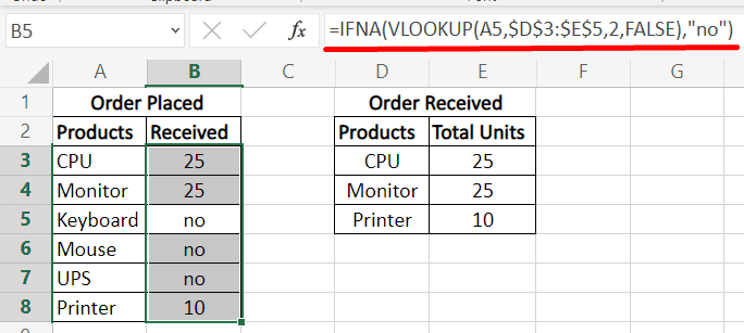
The IFNA function handles only the #N/A error while IFERROR treats all kinds of errors. It returns a custom result when a formula generates the #N/A error, and a normal result when no error is detected. 

IFERROR handles errors that are caused by: 

• wrong formula,
• mistakes in lookup ranges,
• referring to a deleted range,
• forgetting to put quotation marks around a text string in a formula,
• error values from lookup tables

IFERROR replaces all these errors with the value specified in the formula.  

For example, if there’s a typo mistake in the formula, Excel returns #NAME? error, but IFERROR will suppress this and return the value specified in the formula. This might obscure an important problem. It is advisable to use the IFNA function to trap only the #N/A errors.

The following examples show the difference between using an IFNA and an IFERROR function. There is a typo error in the formula as VLOKKUP instead of VLOOKUP. The IFNA function returns a #NAME? error, indicating a mistake in the syntax.

The example below is the same as that above, except that it uses the IFNA function instead of IFERROR to handle the error thrown by the VLOOKUP function. Again, there is a typo error in the function and IFERROR treats it similarly to how it treats other errors and returns the message mentioned in the function.

Suggested Reads: 

Create An Excel Dashboard In 5 Minutes – The Best Guide

Dynamic Dropdown Lists In Excel – Top Data Validation Guide

Predict Future Values Using Excel Forecast Sheet – The Best Guide

Closing Thoughts

In this guide, we explained everything about the IFERROR function in Excel to handle errors in user-defined functions and built-in functions. You can practice using IFERROR inside functions to get a better understanding. But remember to use IFNA when you wish to specifically catch #N/A errors.

We hope that you found this article useful. Please visit our free resources center for more high-quality Excel guides.

Want to learn more about important functions in Excel?

Simon Sez IT has been teaching Excel for over ten years. For a low monthly fee, you can access 130+ IT training courses. Click here for advanced Excel courses with in-depth training modules.

Simon Calder

Chris “Simon” Calder was working as a Project Manager in IT for one of Los Angeles’ most prestigious cultural institutions, LACMA.He taught himself to use Microsoft Project from a giant textbook and hated every moment of it. Online learning was in its infancy then, but he spotted an opportunity and made an online MS Project course - the rest, as they say, is history!