
How to Make a Formula in Excel – Excel Basics
This How to Make a Formula in Excel tutorial is suitable for users of Excel 2013/2016/2019 and Microsoft 365.
OBJECTIVE
Explore Excel functions and create simple formulas from scratch to perform calculations.
FUNCTIONS AND FORMULAS EXPLAINED
If Excel is known for one thing, it’s formulas. Being able to perform simple to very complex calculations by learning how to make a formula in Excel is critical for beginners to understand.
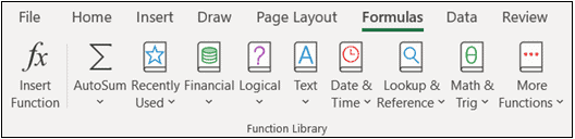
There are over 450 functions in Excel that can be used independently or in combination with other functions to construct simple to complex formulas. Functions are stored in the Functions Library on the Formulas tab, organized by category.
Formulas can be used to add up a list of numbers, find the average of values, count items in a list, make decisions, lookup information and format data. However, there is so much more too them than this.
It can seem intimidating to dive into the world of formulas if you are new to Excel. There are so many that it can seem overwhelming to learn how they work and which will be best for the task. This is something that will come over time with continued practice. However, understanding the basics of how a formula is constructed will give you a great foundation.
HOW TO MAKE A FORMULA – BASIC TERMINOLOGY
First, let’s understand the difference between Formulas and Functions.
| Formulas | A formula is an expression that performs calculations on values in a cell or range of cells. For example, =A1+A2+A3+A4, which finds the sum of the cell range values A1 to A4. |
| Functions | Functions are predefined formulas in Excel. There are 450 functions in Excel. They eliminate the need for the manual entry of formulas. The calculation listed above expressed with a function looks like this: =SUM(A1:A4). The function sums the values in cells A1 to A4. This is a more concise way of writing a formula. |
OPERATORS IN EXCEL
Formulas perform calculations. Much like calculations you used to do in math class, you need to understand how operators work in Excel. An operator is a symbol that denotes if you are adding, subtracting, dividing, or multiplying, amongst other things.
There are many different operators in Excel, so I will highlight the most important ones.
To see a full list visit the Microsoft Support site.
| Operator | Meaning | Example |
| + | Addition | =10+5 |
| – | Subtraction | =10-5 |
| * | Multiplication | =10*5 |
| / | Division | =10/5 |
| > | Greater Than | =A1>B1 |
| < | Less Than | =A1<B1 |
| : | Reference to all the cells between to cell references | =A1:D3 |
INSERTING FORMULAS INTO CELLS
All formulas must begin with an equals (=) sign. That is how Excel knows you want to perform a calculation. Formulas can be typed directly into the cell or in the Formulas Bar.
USING CONSTANTS
In this example, I want to add up the figures for Jan, Feb, and Mar. I could do this using constants, as in, typing the values directly into the cell.

This calculation will produce the correct answer, but it has several drawbacks.
If you are trying to sum lots of numbers, this formula could get very long and difficult to manage. Also, if any of the figures change, the formula would need to be edited.
A much more efficient way of performing this calculation is to use cell references.
USING CELL REFERENCES
In this example, I have replaced constant numbers with cell references. These are the cells that contain the values we want to calculate.
The advantage here is that if any of the figures change, we refer to the cell instead of the actual value so that the result will update automatically.

However, we still have the same problem. If we want to add up many values, this formula will get very long and unwieldy.
A much better way of doing this is to use the SUM function.
USING FUNCTIONS
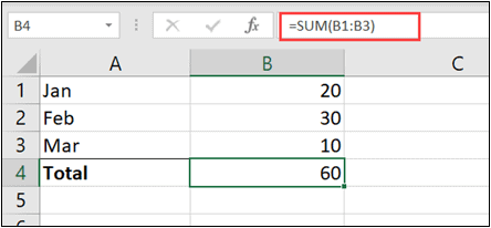
In the below example, we are adding up the figures in cells B1 to B3 using the SUM function in the cell.
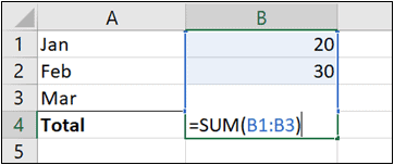
Alternatively, you can type the formula into the Formulas Bar and either click the tick or press Enter to confirm.
INSERTING FORMULAS USING THE FUNCTIONS LIBRARY
If you don’t feel confident entering formulas directly into a cell, you can use the functions dialog box instead.
- Click on the Formulas tab.
- Click Insert Function or press the keyboard shortcut Shift+F3.
- Search for the function you want to use by typing it into the search box, click Go.
- Select the function you want to use.

- Click OK.
- Enter in the cell range you want to sum.
- Click OK.

USING AUTOSUM
A quick way of performing a sum calculation is to use the AutoSum button.
- Click the Home tab.
- From the Editing group, click the AutoSum button. Alternatively, you can press the keyboard shortcut ALT+=
- Press Enter to accept the calculation.

THE BODMAS PRINCIPLE (BIDMAS/PEDMAS)
The BODMAS principle defines the order in which formulas are calculated.
NOTE: BODMAS and BIDMAS are interchangeable names for this rule in the UK. If you are in the US, you may hear this rule referred to as PEDMAS. I learned BODMAS, so that I will be using this in my examples.
Consider the following calculation:
=2+2*10
Without any order of calculation specified, you might assume that you calculate from left to right. In this case, 2+2 = 4, then multiply by 10 to give the result of 40. But this calculation could also be calculated as 2, then add 2 multiplied by 10 to give the result of 22. In its current form, there are two possible answers to this calculation.
We use the BODMAS rule to tell Excel what we want to calculate first.

- Excel will calculate whatever is in brackets (parenthesis) first.
- Next, it will calculate the orders of, square roots, indices, etc.
- It will then calculate divisions or multiplications. If both appear in a formula, it will calculate from left to right.
- Lastly, it will perform any addition or subtractions. If both appear in a formula, it will calculate from left to right.
Let’s modify our formula and add in some brackets (parenthesis).
=(2+2)*10
This time Excel will calculate what’s in the brackets first and then do the multiplication. Written out like this, the answer is 40.
=2+(2*10)
If we move the brackets, we get the answer of 22.
In a more complex calculation where there are two or more pairs of brackets, Excel will calculate the brackets first from left to right.
=(A4+20)/SUM(D5:F5)
So, A4+20 will be calculated first, and then Excel will work out the sum of the values in D5 to F5. Finally, it will divide the result of the sum by the result of A4+20.
In calculations where no brackets are specified, the BODMAS rule will be invoked.
=5+10/2*4
So, according to BODMAS, additions, and subtractions are done at the end. As we also have both a division and a multiplication in this formula, we work from left to right.
First, we calculate 10 divided by 2 to give the result of 5. Then we multiply by 4 to get 20. Finally, we add 5 to give a final result of 25.
We could have made this simpler, by adding brackets.
=5+(10/2)*4
OTHER BASIC FORMULAS
Let’s take a look at some other useful, basic formulas in Excel.
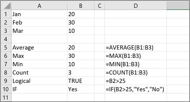
| AVERAGE | The AVERAGE formula calculates the average of the select cell range. |
| MAX | The MAX formula displays the maximum value in a cell range. |
| MIN | The MIN formula displays the minimum value in a cell range. |
| COUNT | The COUNT formula counts the number of items in a selected cell range. |
| LOGICAL | A formula that uses logical operators (>,<,=) will display TRUE or FALSE depending on the logical test result. In this example, I am testing if the value in cell B2 is greater than 25. It is, so the result is TRUE. |
| IF | IF formulas are part of the logical functions group. They perform a logical test and then produce one result if the test is TRUE and one result of the test is FALSE. In this example, I am testing if the value in cell B2 is greater than 25. If it is, then the text ‘Yes’ will be returned. If it isn’t, then the text ‘No’ will be returned’. |
COMBINING FUNCTIONS
In the following example of a more complex calculation, I am combining two functions: SUM and COUNT. Excel works this formula out as follows:
First, if performs a COUNT of cells B1:B3, to give the result of 3.
It then SUM’s cells B1 to B3, to give the result of 60.
Finally, it multiplies the results of the COUNT by the result of the SUM. So, 3 multiplied by 60 to give the result of 180.

Another important point to note when working with formulas is that you must always close as many brackets (parenthesis) as you open. If you forget, Excel will prompt you with a warning message and make the correction for you.
In the above screenshot, notice I have two closing brackets at the end of the formula. The first closes off the B1:B3 argument, and the second closes off the COUNT function.
ABSOLUTE REFERNCING
It’s vital to understand the difference between absolute and relative referencing when working with basic formulas in Excel.
By default, all formulas are calculated using relative referencing.
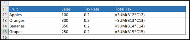
In the example, I have used the SUM formula to multiply the Sales Amount ($) by the Tax Rate to get the total tax payable for each fruit. I have then used the AutoFill handle to copy the formula down for the rest of the fruits.
Notice that as I drag the formula down by default, Excel modifies the cell references, so the calculation for each fruit is correct. This is called relative referencing.
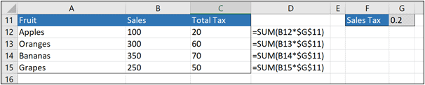
However, as the tax rate is the same each time, the Tax Rate column takes up space. I could put the tax rate in a separate cell on its own and use absolute referencing instead.
In this example, I have deleted the tax rate column and put the tax rate in cell G11. As I want the formula to always refer to the tax rate in cell G11, I have fixed the cell reference using a $ sign in front of the row and the column. You can also use the keyboard shortcut F4 to fix cell references.
As I drag the SUM formula down, the cell reference for the sales will change because I have left that as relative, whereas the cell reference that holds the tax rate will be the same each time I have fixed it (absolute).
These are just a few examples of how to make a formula in Excel. The skills learned here give you a great foundation from which to explore the wonderful world of formulas. If you would like to read more about basic formulas, please check out the following links:
Take a look at the full range of Excel courses from Simon Sez IT
Deborah Ashby
Deborah Ashby is a TAP Accredited IT Trainer, specializing in the design, delivery, and facilitation of Microsoft courses both online and in the classroom.She has over 11 years of IT Training Experience and 24 years in the IT Industry. To date, she's trained over 10,000 people in the UK and overseas at companies such as HMRC, the Metropolitan Police, Parliament, SKY, Microsoft, Kew Gardens, Norton Rose Fulbright LLP.She's a qualified MOS Master for 2010, 2013, and 2016 editions of Microsoft Office and is COLF and TAP Accredited and a member of The British Learning Institute.
